Rolle’s Theorem
Let f be real valued function defined on the closed interval [a, b] such that
It is continuous on the closed interval [a, b].
It is differential on the open interval (a, b) and F (a) = f (b)
Then there exists c ϵ (a, b) such that f’(c) = 0
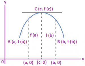
Geometrical Interpretation of Rolle’s Theorem: Let f (x) be real valued function defined on [a, b] such that curve y = f(x) is continuous curve between points A (a, f(a)) and B (b, f(b)). Then ∃ atleast one point (c, f (c)) lying between A and B curve y = f (x) where tangent is parallel to x – axis.
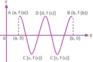
Algebraic Interpretation of Rolle’s Theorem: Let f (x) be polynomial with a and b as its roots. Since polynomial function is everywhere continuous and differentiable and a and b are roots of f (x).
∴ f (a) = f (b) = 0
It states that between any two roots of a polynomial f(x), there is always a root of its derivative f’(x).
Lagrange’s mean value theorem: Let f (x) be a function defined on [a, b] such that
i) It is continuous on [a, b]
ii) It is differentiable on (a, b)
Then ∃ a real number C ϵ (a, b) such that
\(f’\left( c \right)=\frac{f\left( b \right)-f\left( a \right)}{b-a}\).
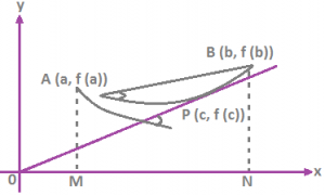
Geometrical Interpretation: Let f(x) be defined on [a, b] such that the curve y = f (x) is a continuous curve between the points A (a, f (a)) and B (b, f (b)) and at every point on the curve, except at the end points, it is possible to drawn a unique tangent. ∃ a point on the curve such that tangent there at is parallel to the chord joining the endpoints of the curve.
Average Rate of Change: If y = f (x) Then average rate of change in y between x = x₁ and x = x₂ is defined as \(\frac{\Delta y}{\Delta x}=\frac{f\left( {{x}_{2}} \right)-f\left( {{x}_{1}} \right)}{{{x}_{2}}-{{x}_{1}}}\),
Instantaneous rate of change of function f at x = x₀
\(f’\left( {{x}_{0}} \right)=\underset{\Delta x\to 0}{\mathop{\lim }}\,\frac{f\left( {{x}_{0}}+\Delta x \right)-f\left( {{x}_{0}} \right)}{\Delta x}\),
s = f (t) where s is the displacement,
\(\frac{\Delta s}{\Delta t}=\frac{f\left( t+\Delta t \right)-f\left( t \right)}{\Delta t}\),
The average velocity between t = t₁ and t = t₂ is \(\frac{f\left( {{t}_{2}} \right)-f\left( {{t}_{1}} \right)}{{{t}_{2}}-{{t}_{1}}}\),
If y = f (x) and x, y is function off then \(\frac{dy}{dt}=f’\left( x \right)\frac{dx}{dt}\),
Errors and Approximations: If a dependent variable y depends on x by a functional relation y = f (x) then change in y is given by Δy = f (x + Δx) – f (x).